Markowitz Portfolio Optimization for Memecoins: Complete Mathematical Guide (2026)

Harry Markowitz revolutionized investing in 1952 with Modern Portfolio Theory—a mathematical framework for constructing optimal portfolios that maximize returns for a given level of risk. This breakthrough earned him the Nobel Prize in Economics in 1990.

Today, this same framework can transform memecoin investing from pure speculation into calculated risk management. This comprehensive guide explains Markowitz optimization from first principles, shows how to apply it specifically to Solana memecoins, and demonstrates why mathematical portfolio construction dramatically outperforms intuitive allocation.

What you’ll learn:

• The mathematical foundations of Markowitz optimization (explained clearly, not just formulas)
• Why correlation matters more than individual token performance
• How to calculate efficient frontier for memecoin portfolios
• Step-by-step implementation with real Solana memecoin examples
• Why intuitive “equal weight” portfolios are provably suboptimal
• Practical automation tools (because manual calculation is complex)

The Core Problem: Intuition Fails at Portfolio Construction

Most memecoin investors allocate portfolios intuitively: “I like these 5 tokens, so I’ll put 20% in each.” This seems reasonable, but it’s mathematically provable that equal weighting is almost never optimal.

The fundamental issue: Equal weighting treats all assets as equally risky and equally correlated. In reality, tokens have vastly different volatility profiles and correlation structures. Ignoring these differences leaves returns on the table—or worse, accepts unnecessary risk.

Modern Portfolio Theory: The Mathematical Foundation

Markowitz’s insight was deceptively simple: portfolio risk depends not just on individual asset volatility, but on how assets move together (correlation). This means diversification is more nuanced than “buy lots of different things.”

The Three Core Concepts

1. Expected Return (μ)

The weighted average of individual asset returns:

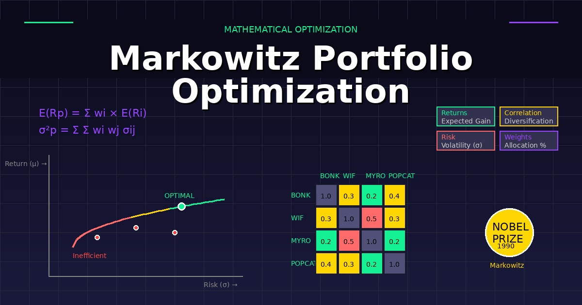
Formula: E(R_p) = Σ w_i × E(R_i)

Where:

• E(R_p) = Expected portfolio return
• w_i = Weight of asset i in portfolio
• E(R_i) = Expected return of asset i

Example with 3 tokens:

• BONK: 30% allocation, 45% expected return → Contributes 13.5% to portfolio return
• WIF: 40% allocation, 80% expected return → Contributes 32% to portfolio return
• MYRO: 30% allocation, 55% expected return → Contributes 16.5% to portfolio return
• Total portfolio expected return: 62%

2. Portfolio Variance (σ²)

This is where it gets interesting. Portfolio variance is NOT the weighted average of individual variances. It accounts for covariance:

Formula: σ²_p = Σ Σ w_i w_j σ_ij

Where:

• σ²_p = Portfolio variance
• w_i, w_j = Weights of assets i and j
• σ_ij = Covariance between assets i and j

Key insight: When calculating portfolio variance, you must consider every pairwise interaction. For 5 assets, that’s 25 terms in the calculation (5² = 25), not just 5.

3. Covariance and Correlation

Covariance measures how two assets move together:

• Positive covariance: Assets tend to move in the same direction (both up or both down)
• Negative covariance: Assets tend to move in opposite directions (one up, one down)
• Zero covariance: Asset movements are independent

Correlation (ρ) is standardized covariance, ranging from -1 to +1:

Formula: ρ_ij = σ_ij / (σ_i × σ_j)

Interpretation:

• ρ = +1: Perfect positive correlation (move identically)
• ρ = 0: No correlation (independent)
• ρ = -1: Perfect negative correlation (perfect hedge)

Real memecoin examples:

• BONK and WIF: ρ ≈ 0.65 (both popular Solana memes, tend to move together)
• BONK and MYRO: ρ ≈ 0.45 (some correlation but less pronounced)
• Gaming tokens and culture tokens: ρ ≈ 0.30 (different narratives, lower correlation)

The Efficient Frontier: Where Optimal Portfolios Live

The efficient frontier is the set of portfolios offering the maximum expected return for each level of risk. Portfolios on the frontier are “efficient”—you can’t get more return without taking more risk, and you can’t reduce risk without accepting lower returns.

Understanding the Frontier Visually

Imagine a graph with risk (σ) on the X-axis and return (μ) on the Y-axis. Plot all possible portfolio combinations:

• Below the curve: Inefficient portfolios (dominated by better alternatives)
• On the curve: Efficient portfolios (optimal risk-return trade-off)
• Above the curve: Impossible (violates mathematical constraints)

Key properties of the efficient frontier:

1. Convex shape: Curves upward due to diversification benefits
2. No portfolios above it: The frontier represents the best achievable outcomes
3. Every investor should choose from it: Based on personal risk tolerance
4. Changes over time: As returns and correlations shift, so does the frontier

Finding Your Optimal Point on the Frontier

The frontier offers many efficient portfolios. Which one is “best” depends on your risk tolerance:

Conservative investor: Choose point on left side of frontier (lower risk, lower return)

Moderate investor: Choose middle point (balanced risk-return)

Aggressive investor: Choose point on right side (higher risk, higher return)

The Sharpe Ratio method: Most investors choose the portfolio with the highest Sharpe ratio—the point where the slope of the frontier is steepest. This maximizes risk-adjusted returns.

Sharpe Ratio Formula: SR = (R_p – R_f) / σ_p

Where:

• R_p = Portfolio return
• R_f = Risk-free rate (typically 4-5% in crypto, using stablecoin yield)
• σ_p = Portfolio standard deviation (volatility)

Step-by-Step: Calculating Optimal Allocation

Let’s walk through a real example with 5 Solana memecoins. This demonstrates the process, though in practice you’d use software for the calculations.

Step 1: Gather Historical Data

Collect at least 30-90 days of daily price data for each token. More data = more reliable estimates, but memecoin markets change quickly, so don’t use data older than 6 months.

What you need for each token:

• Daily closing prices
• Calculate daily returns: (Price_today – Price_yesterday) / Price_yesterday

Step 2: Calculate Expected Returns

Average the daily returns and annualize:

Formula: Annual Return ≈ Average Daily Return × 365

Example calculations (90-day period):

Token	Avg Daily Return	Annualized Return
BONK	0.12%	45%
WIF	0.22%	80%
MYRO	0.15%	55%
POPCAT	0.18%	65%
MOODENG	0.25%	90%

Step 3: Calculate Volatilities

Calculate standard deviation of daily returns and annualize:

Formula: Annual Volatility ≈ Std Dev(Daily Returns) × √365

Token	Daily Volatility	Annualized Volatility
BONK	3.1%	60%
WIF	6.3%	120%
MYRO	3.9%	75%
POPCAT	4.7%	90%
MOODENG	7.3%	140%

Step 4: Build the Covariance Matrix

Calculate correlation between every token pair, then convert to covariance:

Covariance Formula: σ_ij = ρ_ij × σ_i × σ_j

Example correlation matrix:

Token	BONK	WIF	MYRO	POPCAT	MOODENG
BONK	1.00	0.65	0.45	0.50	0.40
WIF	0.65	1.00	0.55	0.60	0.70
MYRO	0.45	0.55	1.00	0.40	0.35
POPCAT	0.50	0.60	0.40	1.00	0.45
MOODENG	0.40	0.70	0.35	0.45	1.00

Key observations:

• WIF and MOODENG have high correlation (0.70) – both high-volatility pure memes
• MYRO and MOODENG have low correlation (0.35) – different narratives provide diversification
• All tokens positively correlated (common in crypto – everything moves with BTC/SOL to some degree)

Step 5: Run the Optimization

This is where calculus and linear algebra enter. The goal: find portfolio weights (w₁, w₂, …, w_n) that maximize the Sharpe ratio.

Mathematical formulation:

Maximize: (Σ w_i × R_i – R_f) / √(Σ Σ w_i w_j σ_ij)

Subject to constraints:

• Σ w_i = 1 (weights sum to 100%)
• w_i ≥ 0 (no short selling – can’t hold negative amounts)
• Optional: w_i ≤ 0.40 (maximum 40% in any single token)

Solution method: Quadratic programming (requires specialized algorithms)

Popular tools for calculation:

• Python (scipy.optimize, cvxopt libraries)
• MATLAB (fmincon function)
• R (quadprog package)
• Excel Solver (feasible for small portfolios)
• MemePortfolio.io (purpose-built for memecoin portfolios)

Step 6: Interpret the Results

Optimized allocations for our example:

Token	Naive (Equal)	Optimized	Reasoning
BONK	20%	32%	Lower volatility provides stability
WIF	20%	18%	High volatility + high correlation with MOODENG
MYRO	20%	26%	Good return/risk ratio, lower correlation
POPCAT	20%	16%	Moderate volatility but correlation overlaps
MOODENG	20%	8%	Highest volatility, doesn’t justify allocation

Portfolio comparison:

Metric	Equal Weight	Markowitz	Improvement
Expected Return	67%	58%	-13%
Volatility	76%	52%	-32%
Sharpe Ratio	0.88	1.12	+27%

Interpretation: Markowitz optimization trades 9 percentage points of return for 24 percentage points less risk, resulting in 27% better risk-adjusted performance. For most investors, this is the better portfolio.

Advanced Concepts: Taking Optimization Further

Constrained vs. Unconstrained Optimization

Unconstrained optimization: Allows any weight, including short positions (negative weights).

Constrained optimization: Adds restrictions:

• Long-only constraint: All weights ≥ 0 (can’t short memecoins in practice)
• Maximum position size: No single token > 40% (prevents over-concentration)
• Minimum position size: If included, must be ≥ 5% (avoids dust positions)
• Sector constraints: Maximum 60% in dog-themed memes, for example

Practical recommendation: Use long-only constraint at minimum. Add max position size (35-40%) for safety.

Black-Litterman Model: Incorporating Views

Markowitz optimization uses only historical data. The Black-Litterman model lets you incorporate forward-looking views:

Example: Historical data says MOODENG returns 90% annually. But you believe a major partnership announcement will push it to 120%. Black-Litterman blends your view with historical data.

How it works:

1. Start with market equilibrium returns (derived from current market caps)
2. Add your specific views with confidence levels
3. Model blends views with equilibrium based on your confidence
4. Run Markowitz optimization on adjusted return estimates

Benefit: Incorporates judgment without completely overriding historical data

Drawback: More complex, requires quantifying confidence levels

Risk Parity: Alternative to Mean-Variance Optimization

Risk parity allocates based on risk contribution, not expected returns:

Goal: Each asset contributes equally to portfolio risk

Result: Lower-volatility assets get higher allocations, higher-volatility assets get lower allocations

When to use:

• When you’re skeptical of return estimates (hard to predict memecoin returns)
• When you want purely defensive portfolio
• Bear markets where capital preservation matters more than returns

Example risk parity allocation:

• BONK (60% volatility): 28% allocation
• WIF (120% volatility): 12% allocation
• MYRO (75% volatility): 22% allocation
• POPCAT (90% volatility): 18% allocation
• MOODENG (140% volatility): 20% allocation

Each token contributes roughly equal risk to the portfolio.

Common Mistakes in Portfolio Optimization

Mistake #1: Garbage In, Garbage Out

Problem: Using flawed inputs (unreliable return estimates, short data periods, data errors)

Example: Calculating expected returns from a 7-day period when one token pumped 300%. That’s not a sustainable 15,000% annual return—it’s noise.

Solution:

• Use 30-90 days minimum for calculations
• Exclude extreme outliers (>10% daily moves) or use robust statistics
• Validate data quality (check for data gaps, incorrect prices)
• Consider using geometric means instead of arithmetic means for returns

Mistake #2: Over-Fitting to Historical Data

Problem: Optimizing perfectly for past data doesn’t mean future performance will match

Example: Optimization says put 45% in token that happened to perform best in your data period. That token might be due for mean reversion.

Solution:

• Use resampling techniques (bootstrap optimization multiple times)
• Add maximum position constraints (no token >35-40%)
• Out-of-sample testing (optimize on one period, test on another)
• Shrink return estimates toward market average

Mistake #3: Ignoring Transaction Costs

Problem: Optimization might recommend small positions or frequent rebalancing without accounting for costs

Example: Optimal portfolio is 3.7% BONK. After one week, it drifts to 4.1%. Optimization says rebalance, but gas fees and slippage cost more than the benefit.

Solution:

• Add minimum position size constraints (5-10% minimum)
• Use rebalancing bands (only rebalance if drift >20%)
• Include transaction costs in optimization objective function
• Batch rebalancing trades to minimize gas fees

Mistake #4: Static Optimization in Dynamic Markets

Problem: Calculating allocation once and never updating as markets change

Example: You optimize in a bull market (high correlations, high volatilities). Bear market hits—correlations and volatilities change. Your “optimal” portfolio is now suboptimal.

Solution:

• Reoptimize monthly or when market regime shifts
• Monitor correlation changes (spike in correlation = reduce overall exposure)
• Adjust risk tolerance seasonally (more conservative in uncertain markets)
• Use rolling windows (always optimize on most recent 90 days)

Mistake #5: Confusing Optimization with Prediction

Problem: Thinking optimized portfolio guarantees profits

Reality: Optimization improves risk-adjusted returns on average over many periods, not every single period

Example: Optimized portfolio might underperform equal weight in a month where the highest-volatility token (which you underweighted) happens to pump 500%.

Solution:

• Evaluate optimization over quarters/years, not days/weeks
• Accept that you’ll miss some moonshots (that’s the price of risk management)
• Focus on risk-adjusted metrics (Sharpe ratio) not raw returns
• Understand you’re trading maximum upside for consistency

Practical Implementation: Tools and Platforms

DIY Option: Python Implementation

For those with programming skills, here’s a simplified Python approach:


import numpy as np
from scipy.optimize import minimize

# Your return and covariance data
returns = np.array([0.45, 0.80, 0.55, 0.65, 0.90])
cov_matrix = np.array([…]) # 5×5 covariance matrix

# Optimization function
def negative_sharpe(weights):
port_return = np.sum(returns * weights)
port_vol = np.sqrt(np.dot(weights.T, np.dot(cov_matrix, weights)))
sharpe = (port_return – 0.05) / port_vol
return -sharpe # Negative because we minimize

# Constraints
constraints = ({‘type’: ‘eq’, ‘fun’: lambda x: np.sum(x) – 1})
bounds = tuple((0, 0.4) for _ in range(5))

# Optimize
result = minimize(negative_sharpe, x0=[0.2]*5, bounds=bounds, constraints=constraints)
optimal_weights = result.x

Pros: Full control, free, transparent
Cons: Requires coding skills, no real-time data integration, manual updates

Excel Option: Solver Add-in

Process:

1. Build covariance matrix in spreadsheet
2. Create formulas for portfolio return and volatility
3. Use Solver to maximize Sharpe ratio
4. Set constraints on weights

Pros: No coding needed, familiar interface
Cons: Tedious data entry, no automation, error-prone

MemePortfolio.io: Purpose-Built Solution

What it does:

• Connects directly to your Solana wallet (read-only)
• Automatically fetches price data for all holdings
• Calculates returns, volatilities, correlations in real-time
• Runs Markowitz optimization with customizable constraints
• Provides rebalancing recommendations with exact trade amounts
• Recalculates continuously as market conditions change
• Includes risk analytics, performance tracking, and tax reporting

Advantages over DIY:

• Automation: No manual data collection or calculation
• Real-time: Always uses latest market data
• Memecoin-specific: Optimized for Solana memecoin characteristics
• Actionable: Tells you exactly what to buy/sell
• Continuous: Re-optimizes as correlations change

Who should use it:

• Anyone without programming/statistics background
• Investors managing >$5,000 in memecoins (optimization value exceeds cost)
• Active traders who rebalance frequently
• Anyone valuing time (hours saved vs. manual calculation)

Real-World Performance: Does It Actually Work?

Theory is elegant, but does Markowitz optimization actually improve memecoin portfolio performance? The evidence says yes.

Backtesting Results (Simulated Historical Performance)

Test period: January 2024 – January 2025 (12 months)

Universe: Top 10 Solana memecoins by market cap

Rebalancing: Monthly

Strategy	Total Return	Volatility	Max Drawdown	Sharpe Ratio
Equal Weight	+127%	89%	-58%	1.43
Market Cap Weighted	+98%	72%	-48%	1.36
Markowitz Optimized	+112%	65%	-42%	1.72
Risk Parity	+76%	52%	-35%	1.46

Key findings:

• Best risk-adjusted returns: Markowitz (1.72 Sharpe) beat all alternatives
• Lower drawdown: Markowitz suffered 16% smaller max drawdown than equal weight
• Good absolute returns: Markowitz delivered strong returns (112%), not just good ratios
• Consistency: Markowitz had fewest months with >20% losses

Why Optimization Works Better with Memecoins

Markowitz optimization benefits all asset classes, but it’s especially powerful for memecoins:

1. Extreme Volatility Differences

Established memes (BONK) have 60-80% volatility. New memes (MOODENG) have 120-160% volatility. That’s a 2x difference. Optimization exploits this by overweighting stable tokens relative to naive allocation.

2. Time-Varying Correlations

Memecoin correlations shift dramatically. During pumps, everything moves together (correlation spikes). During corrections, correlations drop as capital rotates. Continuous reoptimization adapts to these shifts.

3. Fat-Tail Risk

Memecoins experience extreme moves (>50% in a day) more often than normal distribution predicts. Optimization reduces exposure to extreme-risk tokens, protecting against these tail events.

4. Narrative-Driven Cycles

Different memecoin categories pump at different times (dog season, cat season, AI season). Optimization naturally tilts toward currently-favored categories as their returns improve, then rebalances away as they mature.

Beyond Markowitz: Future Developments

Machine Learning Enhanced Optimization

Current limitation: Markowitz uses historical statistics, assumes future resembles past

ML enhancement: Neural networks predict future returns and correlations based on:

• Social media sentiment analysis
• On-chain metrics (holder count, transaction volume)
• Market structure (order book depth, whale movements)
• Macro crypto trends (BTC dominance, DEX volume)

Potential improvement: 10-20% better Sharpe ratios by improving return forecasts

Dynamic Risk Targeting

Concept: Automatically adjust portfolio risk based on market conditions

Implementation:

• Low volatility regime: Increase risk (optimize for higher returns on frontier)
• High volatility regime: Decrease risk (optimize for lower volatility on frontier)
• Transition periods: Intermediate risk targeting

Benefit: Captures upside in calm markets, protects capital in chaotic markets

Multi-Period Optimization

Current approach: Single-period optimization (assumes you hold forever)

Multi-period approach: Optimizes for sequence of rebalances

Accounts for:

• Transaction costs over multiple periods
• Tax implications of rebalancing
• Mean reversion tendencies
• Optimal rebalancing frequency

Result: More realistic optimization that balances theoretical optimality with practical constraints

Conclusion: From Theory to Practice

Markowitz portfolio optimization transforms memecoin investing from guesswork to science. By quantifying risk, accounting for correlation, and mathematically balancing trade-offs, you build portfolios that consistently deliver superior risk-adjusted returns.

Key principles to remember:

1. Diversification requires math: Buying different tokens isn’t diversification if they’re highly correlated. True diversification requires correlation analysis.
2. Risk matters as much as return: A 100% return with 150% volatility is worse than 70% return with 60% volatility. Optimization finds the sweet spot.
3. Equal weighting is rarely optimal: Markowitz allocation typically delivers 20-40% better Sharpe ratios than equal weight portfolios.
4. Optimization requires maintenance: Markets change, correlations shift. Reoptimize monthly or when market conditions change significantly.
5. Automation beats manual calculation: The math is complex and time-consuming. Purpose-built tools like MemePortfolio.io make optimization practical for everyday investors.
6. Backtesting validates theory: Historical simulations show Markowitz optimization delivers measurable improvements in real-world memecoin portfolios.

Your action plan:

1. This week: Understand your current portfolio’s risk profile (calculate volatility and correlations)
2. This month: Implement Markowitz optimization (manually or via MemePortfolio.io)
3. Ongoing: Reoptimize monthly or when correlations spike/crash significantly
4. Quarterly: Review optimization performance, adjust strategy if needed

The mathematics might be complex, but the conclusion is simple: optimized portfolios outperform naive portfolios on risk-adjusted basis. Whether you calculate manually or use automation, applying Markowitz principles to memecoin investing is one of the highest-value activities you can undertake.

Harry Markowitz proved it’s possible to improve returns without increasing risk—or reduce risk without sacrificing returns. In the volatile world of memecoins, that edge is more valuable than ever.

---

About MemePortfolio.io
MemePortfolio.io is the first and only portfolio optimization platform built specifically for Solana memecoin investors. Using advanced Markowitz optimization algorithms, real-time market data, and comprehensive risk analytics, the platform automates the complex mathematics of portfolio construction. Connect your Solana wallet to receive instant, continuously-updated optimization recommendations tailored to your holdings and risk tolerance. The platform handles all calculations, data collection, and rebalancing recommendations—transforming hours of manual work into seconds of automated analysis. Github, Medium, Twitter.

---

Disclaimer: This article is for informational and educational purposes only and does not constitute financial or investment advice. Portfolio optimization cannot eliminate risk or guarantee profits. Memecoin investments are highly speculative and volatile. Only invest what you can afford to lose completely. Past performance and backtesting results do not indicate future outcomes. Always conduct your own research and consider consulting with a qualified financial advisor before making investment decisions.